June 2024
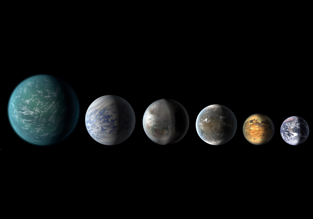
Artist's Concept of a Pantheon of Exoplanets that are similar to Earth
5 conceptual exoplanets plus Earth at the far right.
Credit: NASA
Introduction
An exoplanet (also known as an extrasolar planet) is a planet outside of our Solar System. Exoplanets hold
fascination since an exoplanet is the most likely location for life elsewhere in the universe. For
millennia, one of the most fundamental questions posed by humans has been "Are we alone?" By studying
exoplanets, we can learn how solar systems form and we can determine how common, or rare, are the conditions
of our Solar System and our planet Earth. The primary goal for a future NASA flagship astrophysics mission
is to find biosignatures in the atmospheres of Earth-like exoplanets orbiting Sun-like stars within 200
light-years of Earth. We will discuss that mission - the Habitable Worlds Observatory - in the July 2024
article. This article focuses on the main methods by which we discover and measure the basic properties of
exoplanets.
The First Exoplanet Discovery - Pulsar Timing
While news stories about exoplanets appear on a weekly and sometimes daily basis, it is important to
remember that exoplanet science is a very recent field of research. The first exoplanet discovery was
announced just 32 years ago, in 1992, by Aleksander Wolszczan, a Polish astronomer working at Pennsylvania
State University, and Dale Frail, a Canadian astronomer working at the National Radio Astronomy Observatory
(New Mexico).
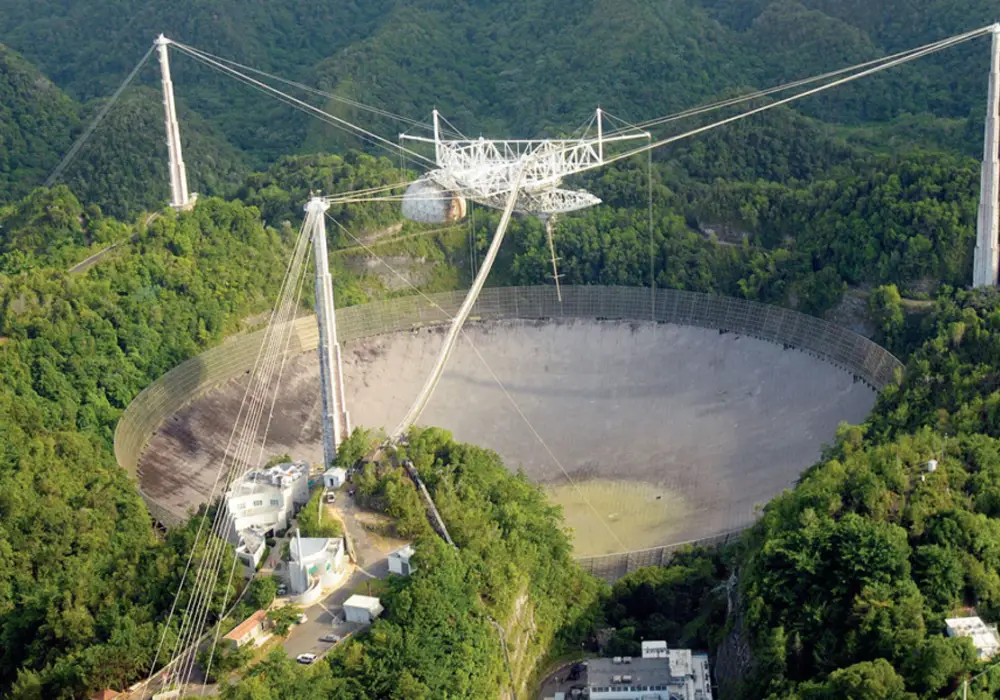
305-meter diameter Arecibo Telescope (Puerto Rico)
Operational for 57 years (1963 -
2020). The receiver and radar transmitters are mounted 150 meters above the dish.
Credit: Wikipedia
In 1990, Wolszczan and Frail used the Arecibo Radio Observatory in Puerto Rico to discover a pulsar that is
named PSR B1257+12. A pulsar, which is the small, ultra dense remnant of a star that exploded as a
supernova, emits radio waves extremely regularly as it rotates. If a planet orbits the pulsar, the planet
will cause slight anomalies in the timing of the pulsar's observed radio pulses. In 1992, Wolszczan and
Frail announced that the pulsar was orbited by two planets; the exoplanets have been named Poltergeist and
Phobetor. Pulsars do not provide hospitable environments for life on their exoplanets and pulsar timing has
not been a productive method to find exoplanets. To date, only 7 exoplanets have been found orbiting
pulsars. This may be because when the star went supernova (and produced the pulsar) the supernova explosion
would likely have destroyed any planets orbiting the progenitor star. Thus, any exoplanets orbiting pulsars
are probably "second generation" that formed after the supernova explosions.
The quest for discovery of exoplanets that may be hospitable to life has focused on stars that are on the
"main sequence". To understand exoplanets and the habitable zone of exoplanets, it is useful to review the
evolution of stars.
The Main Sequence of Stellar Evolution
Stars are formed by the gravitational collapse of gas and dust. As the mass of a protostar increases,
its gravity increases pressure which in turn increases temperature. After millions of years, the core
temperature of the protostar reaches conditions at which nuclear fusion can begin. The star then begins
the longest stage of its life, called the main sequence. Most stars in our Milky Way galaxy,
including our Sun, are categorized as main sequence. During the main sequence, nuclear fusion in the
star converts hydrogen into helium. This fusion process releases energy that keeps the star hot and
bright, and supplies an outward pressure against the incredible mass of material that would otherwise
cause the star to collapse on itself. Ninety percent of a star's life is spent in the main sequence
phase.
Stars have a huge range of brightness, also called magnitude. The brightness of stars, as seen from
Earth, depends on distance; light intensity falls off as the square of the distance from the star to the
observer. The apparent brightness of a star as seen from Earth is the apparent magnitude. The
brightest stars are first magnitude, the next brightest stars are second magnitude, and so on. The
dimmest stars visible to the naked eye in a very dark location are about 7th magnitude. One
of the earliest record of stars listed by apparent magnitude was done by the ancient Roman astronomer
Claudius Ptolemy (who lived during 100-170 AD). Ptolemy's star catalog listed stars from 1st
to 6th magnitude. Since the brightness assessment was done by the human eye which has a
logarithmic response, each magnitude corresponds to a reduction of brightness by a multiplicative
factor. In 1856, the English astronomer Norman Robert Pogson noticed that 6th magnitude stars
are almost exactly 100 times fainter than 1st magnitude stars. Pogson recommended that
astronomers quantify each step in magnitude as the fifth root of 100 in brightness (1001/5),
or a factor of 2.512. Astronomers now use Pogson's ratio as the formal relation for the magnitude
scale.
Magnitude is a reverse logarithmic scale; whereby smaller numbers denote brighter objects. The
1st magnitude stars are not the brightest objects in the sky. Jupiter is magnitude -2.7, and
Venus at its brightest is magnitude -4.6. The full Moon has a magnitude of -12.6 and the Sun is
magnitude -26.7. Using Pogson's ratio we can compute that Jupiter and Venus are respectively 30 and 174
times brighter than 1st magnitude stars. The Moon is 275,592 times brighter than a
1st magnitude star, and the Sun is 120 billion times brighter than a 1st magnitude
star.
Telescopes have large apertures and can integrate light for hours to image very faint objects. One of
the deepest images taken by the Hubble Space Telescope is the Hubble eXtreme Deep Field (XDF), which is
the result of co-adding 2 million seconds of exposures (about 23 days) collected over 10 years. The
faintest objects seen in the Hubble XDF are about magnitude 31, nearly 4 billion times fainter than the
faintest stars visible to a human's naked eye.
When comparing the brightness of celestial objects, astronomers scale the apparent magnitude seen at
Earth to the brightness of the object as it would be when observed from a distance of 10 parsec (32.6
light years). This value, called absolute magnitude, is the luminosity that a celestial object emits, a
much more useful quantity when comparing objects. The absolute magnitude of a star is related to how
much energy it produces.
Stars also vary in color because they vary in temperature. Hotter stars appear blue or white, while
cooler stars look orange or red. Astronomers use these characteristics to classify main sequence stars
into categories defined by color and temperature, from hottest and largest to the coolest and smallest:
O (blue), B (blue-white), A (white), F (yellow-white), G (yellow), K (orange), and M (red). Our Sun is a
G-type star.
Astronomers plot the main sequence on a graphic called the Hertzsprung-Russell diagram (shown
below). Also called the H-R diagram or the color-magnitude chart, this chart has been used by
astronomers since the early 20th century. In 1911, Danish astronomer Ejnar Hertzsprung made a chart of
stellar magnitudes (brightness) and colors. Two years later, Henry Norris Russell showed that stars
could be put into groups based on their luminosity and temperature. The chart is named after both
scientists. The H-R diagram is very useful since it can be used to chart the life cycle of a star.
In the Hertzsprung-Russell diagram the temperatures of stars (colors) are plotted against their
luminosities. Note that both scales are logarithmic, to cover a wide range of values. Stellar brightness
is scaled relative to the brightness of our Sun (which has a brightness value of 1 in the H-R diagram).
The position of a star in the diagram provides information about its present stage and its mass. Stars
that burn hydrogen into helium lie on the diagonal branch, which is termed the main sequence.
Stars in the main sequence (which includes the Sun) plot in a band which runs from the top-left to the
bottom-right of the H-R diagram. The H-R diagram shows that the temperature of main-sequence stars
increases with brightness. This is because the star's mass controls both its temperature and brightness
during the main sequence stage.
Red giant and red supergiant stars fall in the top-right of the chart. This tells us they
are brighter than main sequence stars but also redder and cooler. This is because they expand and cool
as they reach the final stages of their lives. However, because of their large size, they remain very
bright.
In the bottom-left of the chart, we find hot stars that are dimmer than main-sequence stars. This is
because they have small radii but contain a lot of mass. These are white dwarf stars.
Stars tend to spend about 90% of their life in the main sequence stage, and most of the main sequence
stage is spent in the red dwarf stage at the end of the star's life. About 6% of the Milky Way stars are
like our Sun, a G-type (yellow) star. About 13% of Milky Way stars are orange dwarfs (K-type) and about
73% of Milky Way stars are red dwarfs (M-type).
After the main sequence, stars evolve into giant stars for the remaining 10% of their lives. Finally,
red giants will either explode as a supernova or become white dwarf stars.
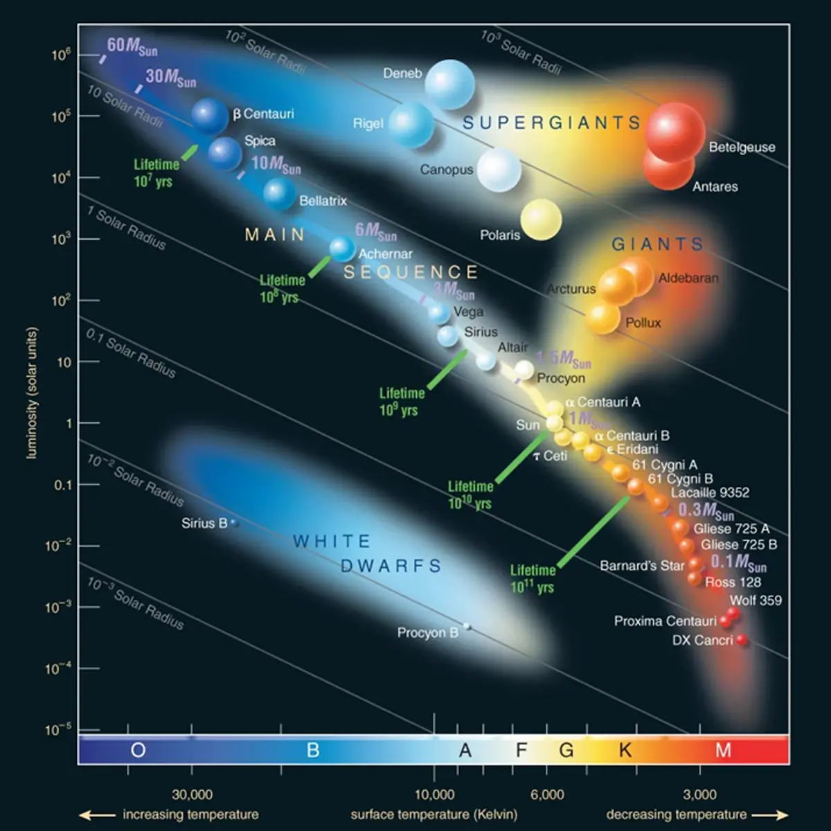
Hertzsprung-Russell Diagram
Credit: Pearson Education, Inc. publishing as Pearson Addison-Wesley (2008)
-
Temperature is plotted on the x-axis (horizontal axis) with hotter stars to the left (30,000 K
surface temperature) and cooler stars toward the right (3,000 K).
-
Absolute stellar brightness (luminosity) is plotted on the y-axis (vertical axis) with the brightest
stars at the top. Brightness is scaled relative to the Sun (which has value of 1 on this plot).
-
Familiar stars on the H-R diagram are
- the Sun (G-type, relative luminosity of 1)
- Betelgeuse (M, 105) - the red star in the "left shoulder" of the Orion constellation
- Proxima Centauri (M, 10-3) - the closest star to our Sun, and
- Sirius (A, 25) - the brightest star seen in the night sky.
Note that many objects cannot be plotted on the H-R diagram due to their extreme and complex properties
- such as neutron stars, pulsars, and black holes.
-
Neutron stars and pulsars are the stellar cores of supergiants that have collapsed. They have
temperatures of approximately a million degrees Kelvin and are far too hot to be plotted on the H-R
diagram.
-
Black holes emit no light of their own and therefore have no absolute visual magnitude.
The Radial Velocity Method for Detecting Exoplanets
Advancements made in spectrometer technologies and observational techniques during the 1980s enabled a new
technique to discover exoplanets around main sequence stars. Astronomers began to precisely measure the
wavelengths emitted by a star to determine if an exoplanet was causing the star to "wobble" about the
barycenter (center of mass) of the star-planet system. This technique is based on measuring the light of the
star. The planet is a hidden companion which is indirectly detected by measuring the gravitational effect of
the planet on the star's motion. This approach, called the radial velocity method, is shown in the
animation below.
Animation of the radial velocity method for finding exoplanets
A star and its companion planet both orbit the barycenter (center of mass), which results in a small
"wobble" of the star (top left). When viewed edge-on (bottom left), the star moves periodically
towards and away from an observer (in the direction in and out of the page). This radial speed (top
right) can be measured using doppler spectroscopy, which is a technique that splits the star's light
into a spectrum of different colours. Absorption lines in the spectrum are due to chemicals in the
star's atmosphere, and their exact colors are determined by the chemical structure. The radial speed
of the star causes a doppler shift of the star's light, which can be detected if the absorption
lines are different from their expected value (bottom right).
Credit: Alysa Obertas (own work, 12 July 2022)
This image is licensed under the Creative Commons Attribution-Share Alike 4.0 International license.
To pursue discovery of exoplanets, the Observatoire de Haute-Provence installed the ELODIE echelle
spectrograph at their 1.93 meter telescope in southeastern France, achieving first light in 1993. The
spectrograph was placed in a temperature controlled room to minimize flexure due to gravity and
expansion/contraction due to temperature changes. Visible light (389.5 to 681.5 nm) from stars was supplied
to the ELODIE spectrograph using optical fibers mounted at the Cassegrain focus of the telescope. The ELODIE
instrument was able to measure radial velocities to an accuracy of ±7 m/sec.
On October 6, 1995, Swiss scientists Michel Mayor and his graduate student Didier Queloz at the University
of Geneva, announced at a conference in Florence, Italy that the ELODIE spectrograph was able to discover
the first exoplanet orbiting a main sequence star located 50 light-years from Earth, 51 Pegasi.
For this discovery, Mayor and Queloz were awarded half of the 2019 Nobel prize in Physics. Their Nobel
prize was shared with James Peebles, a Canadian-American astrophysicist who is widely regarded as one of
the world's leading theoretical cosmologists.
The exoplanet, named 51 Pegasi b, is a "hot Jupiter" (large gas planet) orbiting very close to its host
star. The orbit of 51 Pegasi b is only 4.3 days. On the west coast of the United States, two American
astronomers, Geoff Marcy and Paul Butler, were also using the radial velocity method to search for
exoplanets. One week after Mayor and Queloz made their announcement, Marcy and Butler confirmed the 51
Pegasi b discovery using an echelle spectrograph at the Lick Observatory 3-meter telescope in California.
Telescope that Michel Mayor and Didier Queloz used to discover the first exoplanet orbiting a main
sequence star
Left: 1.93-meter telescope at Observatoire de Haute-Provence (France) - 650-meter (2,133 ft)
altitude
Right: The 1.93-meter telescope shown with dome open and dome lights on.
- The ELODIE spectrograph was placed in a temperature-controlled room on the first floor of the 1.93-m
telescope building. Light from stars was captured by optical fibers mounted at the Cassegrain focus
(back end of the telescope shown at left). The fibers were routed down to the ELODIE spectrograph.
Photos courtesy of Observatoire de Haute-Provence (OHP) / Centre National de la Recherche Scientifique
(CNRS)
The race was on to find more exoplanets, and the floodgates of discovery were opened. Marcy and Butler
announced their first exoplanet discoveries in January 1996, around the stars 70 Viginis and 47 Ursae
Majoris. These exoplanets had orbits closer to what we have in our Solar System, with orbital periods of 116
days and 2.5 years. During the next few years, Marcy and Butler used spectrographs at Lick Observatory and
the Keck Observatory (in Hawai'i) to discover at least 70 of the 100 exoplanets found by the radial velocity
method in the 1990's.
Telescopes that Geoff Marcy and Paul Butler used to discover exoplanets with the radial velocity method
Left: Lick Observatory 3-meter Shane Telescope (California) - 1,283-m (4,209 ft) altitude
Right: Keck I and Keck II 10-meter telescopes (summit of Mauna Kea, Hawai'i) - 4,145-m (13,600 ft)
altitude
Photos courtesy of University of California Regents / Ethan Tweedie Photography
During the last 30 years, nearly every major ground-based telescope has installed a high precision spectrograph
for searching for exoplanets with the radial velocity method. Through 2023, the radial velocity method has
discovered over 1,000 exoplanets, about 20% of the >5,000 exoplanets confirmed.
Most of the radial velocity spectrographs operate in the visible (a.k.a. "optical") using high performance CCDs
supplied by Teledyne e2v Space Imaging (Chelmsford, UK) to detect the light. Precise Doppler spectroscopy is
most easily done in the optical since:
- wavelength measurement is well calibrated,
- optical detectors are better behaved and more easily calibrated than infrared detectors, and
- absorption and emission from the Earth's atmosphere is easier to correct in the optical than it is in the
infrared.
Over the past 10 years, an increasing number of radial velocity spectrographs have been developed for the
infrared due to the following reasons:
- The vast majority of stars in the Milky Way - about 73% - are M-type stars which emit their maximum light
flux in the infrared.
- It is easier to find planets that are in the habitable zone around cool M-dwarf stars. The Habitable
Zone is the range of orbital radii within which the exoplanet surface can support liquid water given
sufficient atmospheric pressure.
- Sometimes the habitable zone is referred to as the Goldilocks Zone, an allusion to the
children's fairy tale of "Goldilocks and the Three Bears", in which a little girl chooses from sets
of three items. When choosing porridge, she chose the porridge that was "not too hot and not too
cold".
- Since M-stars are cool, the habitable zone is close to the star, and exoplanets in the habitable zone around
M-stars have shorter periods than G-type (Sun-like) and K-type stars.
- Exoplanets around M-stars also can have a larger exoplanet to star mass ratio. Combined with the closer
orbits of the habitable zone, the star's wobble is much larger, and the precision of an infrared radial
velocity spectrograph does not have to be as good as the optical spectrographs.
Most of the infrared radial velocity spectrographs use the H2RG or H4RG-15 infrared focal plane arrays produced
by Teledyne Imaging Sensors (Camarillo, California).
Today, the state-of-the-art in high precision radial velocity spectrographs is represented by the HARPS and
ESPRESSO spectrographs of the European Southern Observatory (ESO). Both HARPS and ESPRESSO are stable with
precision below 1 m/sec, with ESPRESSO aspiring to 0.1 m/sec precision. This is a large improvement over the 7
m/sec precision achieved by the ELOIDE spectrograph that discovered the first exoplanet orbiting a main sequence
star in 1995.
The High Accuracy Radial-velocity Planet Searcher (HARPS) spectrograph was designed with every possible feature
to enable it to measure radial velocities with high accuracies over long term observations. To achieve the goal
of 1 meter/sec accuracy over extended periods, the HARPS spectrograph is housed within a vacuum vessel buried
within the building of the 3.6-meter telescope at the La Silla Observatory that is operated by the European
Southern Observatory (see image below). The vacuum vessel enables the spectrograph to avoid spectral drift due
to temperature and air pressure variations. The temperature is further stabilized by placing the vacuum vessel
in a temperature controlled room with human access only during maintenance periods. Starlight is fed to the
spectrograph by optical fibers mounted at Cassegrain focus of the 3.6-meter telescope.
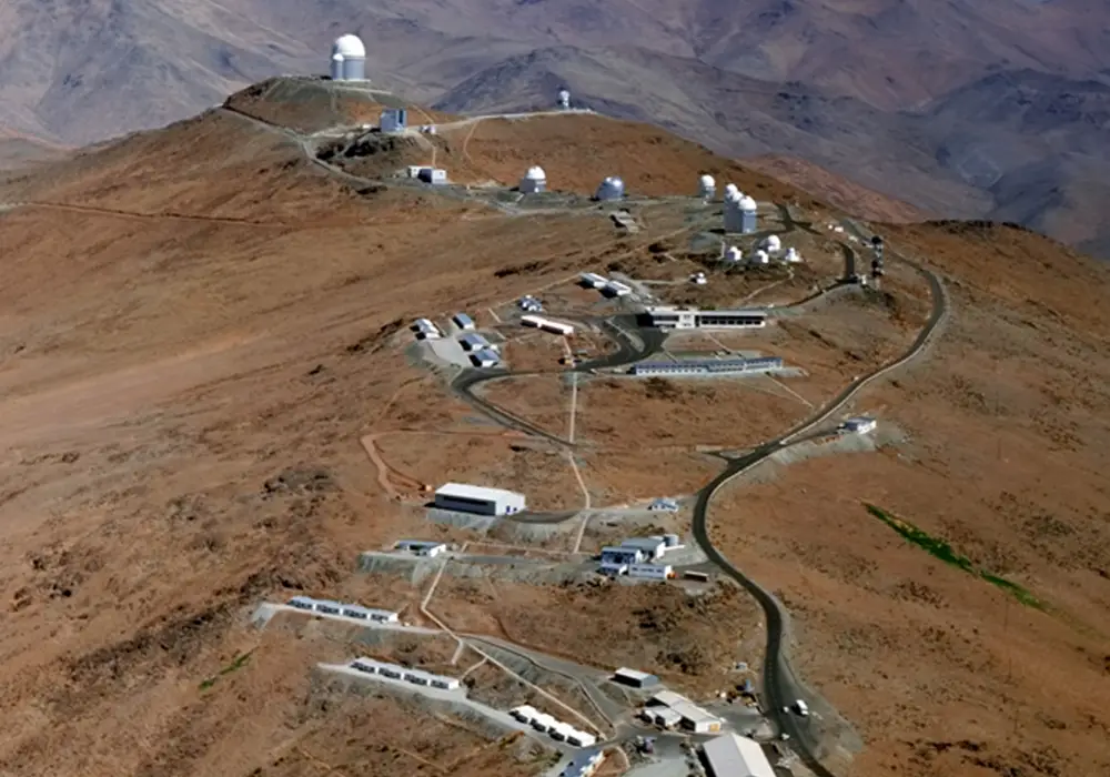
La Silla Observatory (Chile)
3.6-meter telescope located at the top of the ridge (at the top of this
image). La Silla is operated by the European Southern Observatory (ESO).
Credit: ESO
The HARPS spectrograph uses two Teledyne e2v 2048x4102 pixel CCDs (15 µm pitch) to sense light over the 378
- 691 nm band (near UV through red). An example of this CCD, named EEV44-82, is shown below in the CCD test
dewar at ESO Headquarters (Garching, Germany). The HARPS vacuum vessel is shown while being tested at the Geneva
Observatory (Switzerland).
HARPS radial velocity spectrograph - optical focal plane array (CCD) and vacuum vessel
HARPS uses two of the EEV44-82 CCDs (one shown under test at left). At right, the HARPS spectrograph vacuum
vessel is shown under test at Geneva Observatory before shipment to Chile.
Credit: ESO
There are advantages and drawbacks for the radial velocity method for discovery of exoplanets.
- Advantages
- The radial velocity method is ideal for ground-based telescopes since observations do not need to be
made continuously as required for transit photometry (discussed in the next section).
- The radial velocity measurement is not dependent on the distance to the star (with the caveat that stars
get fainter the farther the stars are from Earth). Radial velocity could be used for stars across the
Milky Way galaxy if those stars were sufficiently bright.
- Drawbacks
- A fundamental feature of the radial velocity method is that it cannot accurately measure the mass of an
exoplanet; it only provides an estimate of the exoplanet's minimum mass. This is because radial velocity
only measures the motion of stars towards and away from Earth. This is not a problem if the orbital
plane of the exoplanet appears edge-on when observed from Earth. But most exoplanet orbits are tilted
relative to the direction to the Earth and the "wobble" of the star is decreased by the sine of the
angle between direction toward the Earth and the orbital plane of the exoplanet. This sin(i)
term, where i denotes the orbit inclination, reduces the observed wobble and decreases the
derived exoplanet mass.
- A second drawback of the radial velocity method is that it is biased toward finding large exoplanets
orbiting smaller M-type stars. These exoplanets are unlikely abodes for life.
- Lastly, there is a practical limit to the sensitivity of radial velocities since stars have features and
convective cells that produce noise on the velocity measurements of the star. Depending on the type of
star, this noise can be more than 1 meter/sec. Our Sun is a relatively quiet star but it still produces
radial velocity scatter due to sunspots at the level of 50 cm/sec (0.5 m/sec). While that may seem
small, the radial velocity signal that the Earth has on our Sun is only 10 cm/sec (0.1 m/sec). No
matter what advancements are made during the next 20 years, astronomers do not expect to be able to use
the radial velocity method to detect Earth analogue exoplanets.
Radial velocity measurements opened the field of exoplanet discovery and, through 2023, the radial velocity method
has discovered over 1,000 exoplanets. However, the greatest number of exoplanets have been discovered using a method
termed "transit photometry" which is explained in the next section.
The Transit Photometry Method for Detecting Exoplanets
Viewed from Earth, if the orbital plane of exoplanets are seen edge on, the exoplanet can be detected by measuring
the brightness of the star over time to see a dip in brightness when the exoplanet transits its host star. A larger
exoplanet will create a larger dip in brightness. This is shown in the animation below.
Animation of a transit of a small rocky planet followed by a transit of a gas giant planet
The light curves appear at the bottom of the animation. The horizontal axis represents time, the vertical
axis represents the brightness of the star. The dips that are measured are typically at most a few % of the
star's intensity.
Credit: NASA Goddard Space Flight Center
There is a dip in brightness when the exoplanet passes in front of the star, and also when the exoplanet passes
behind the star, i.e. the exoplanet is occulted by the star. This is shown in the graphic below.
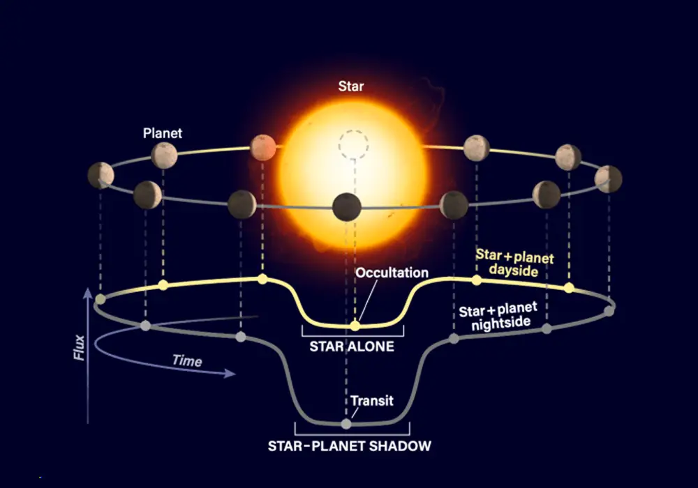
Transit Photometry Method for finding exoplanets
The transit method finds exoplanets by looking for dips in starlight as the exoplanet passes between Earth
and its host star. However, this only works when the star and exoplanet happen to line up as we see them
from Earth. Because stars and planets are oriented randomly in space, not all exoplanets have orbits that
carry them in front of their stars from our point of view.
Credit: Astronomy: Roen Kelly
The transit photometry approach for finding exoplanets measures the total brightness of the star + exoplanet.
If the light from star + exoplanet is fed to a spectrograph, this approach can be expanded to transit
spectroscopy. Accurate measurements of the spectra from star alone (planet behind the star), star plus
exoplanet (planet to the side of the star), and exoplanet in front of the star can be processed to isolate the
exoplanet spectrum from the host star spectrum. Transit spectroscopy is being attempted with the James Webb Space
Telescope; preliminary results have been mixed.
Ariel: In 2029, the European Space Agency (ESA) will launch a mission that is optimized for transit
spectroscopy: the Atmospheric Remote-Sensing Infrared Large-survey (Ariel) mission. Ariel will be located at
Lagrange Point L2 and will perform a chemical census of the atmospheres of 1000 transiting exoplanets. The Ariel
mission will focus on exceptionally hot planets in our galaxy, with temperatures greater than 600 degrees Fahrenheit
(320 degrees Celsius). Such planets are more likely to transit their star than planets orbiting farther out, and
their short orbital periods provide more opportunities to observe transits in a given period of time. More transits
give astronomers more data, allowing them to reveal the weak chemical fingerprint of a planet's atmosphere.
Ariel's hot exoplanet population will include gas giants like Jupiter, as well as smaller gaseous planets called
mini-Neptunes and rocky worlds bigger than our planet called super-Earths. While these planets are too hot to host
life as we know it, they will tell us a lot about how planets and planetary systems form and evolve. Additionally,
the techniques and insights learned in studying exoplanets with Ariel will be useful when scientists use future
telescopes to look toward smaller, colder, rockier worlds with conditions that more closely resemble Earth's.
Artist concept of the Ariel spacecraft and payload
Credit: ESA
Ariel will perform observations in three photometric bands (0.5-0.6 µm, 0.6-0.8 µm, and 0.8-1.1 µm)
and three spectroscopic bands: 1.1-1.95 µm, 1.95-3.9 µm, and 3.9-7.8 µm. Ariel
will simultaneously measure all wavelengths in the 0.5-7.8 µm spectral range.
Ariel will use infrared focal plane arrays that were produced by Teledyne Imaging Sensors (Camarillo, California).
Ariel will use three substrate-removed SWIR (2.3 µm λco) H2RG focal plane arrays (FPAs) for the
photometric bands and the shortest wavelength spectroscopic band. The SWIR H2RG FPAs will be operated by SIDECAR
ASIC modules. These SWIR H2RG FPAs and SIDECAR ASIC modules are residual from ESA's Euclid mission. Ariel will use
two H1RG FPAs, with cutoffs of 4.8 and 8.2 µm, for the 1.95-7.8 µm spectroscopic bands. The H1RG FPAs will
be actively cooled by a Joule-Thomson system to an operating temperature of 42K.
The transit photometry approach has discovered most of the exoplanets found to date. This success is primarily due
to two NASA space missions - Kepler and TESS - which are explained below.
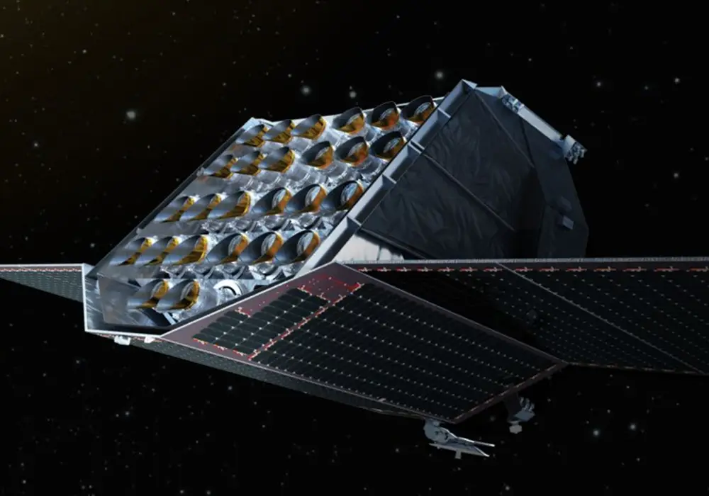
Kepler: The Kepler mission was NASA's first planet-hunting mission to use transit photometry. Launched
on March 6, 2009, Kepler combined cutting-edge observational techniques for measuring stellar brightness with the
largest digital camera outfitted for space at that time. Kepler used a large focal plane mosaic (shown below) that
was outfitted with 25 modules mounted on a curved surface to optimize the instrument focus. (Although it is hard
to see in the image, each module is flat.) There are 21 modules with image arrays used for measuring the
brightness of stars, and four corner modules used for measuring guide stars to maintain accurate telescope pointing.
The focal plane mosaic was assembled by Ball Aerospace in Boulder, Colorado. (Ball Aerospace was acquired by BAE
Systems in February 2024.)
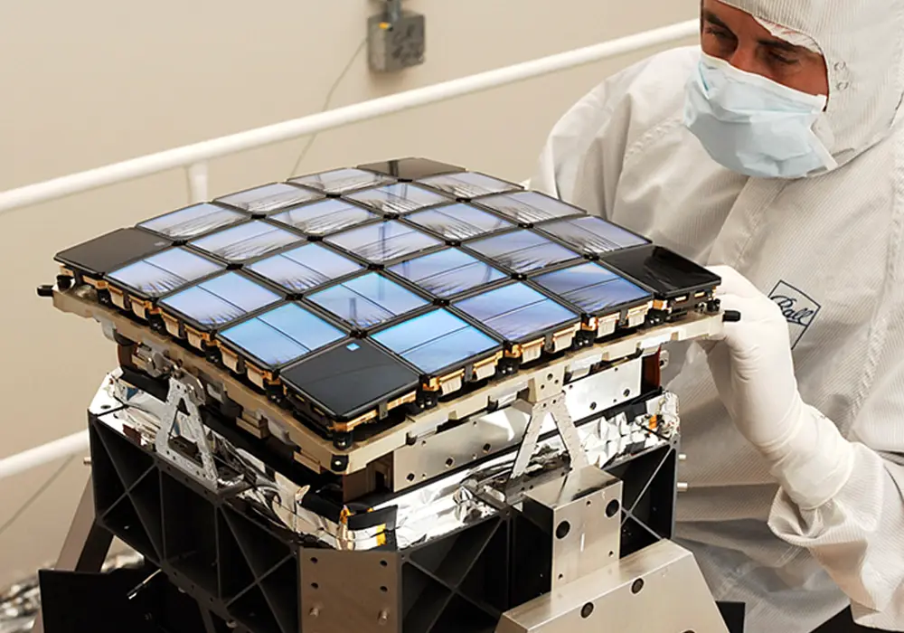
Kepler Focal Plane
The Kepler focal plane is composed of 25 individually mounted modules. The four corner modules are used for
fine guiding and the other 21 modules are used for science observations. Note that the four fine guidance
modules in the corners of the focal plane are much smaller CCDs than the science modules. Each module and
its electronics convert light into digital numbers that are analyzed for exoplanet transits.
Credit: NASA
Each of the 21 science modules uses two charge coupled devices (CCDs) produced by Teledyne e2v Space Imaging in
Chelmsford, UK. Each CCD has 2200x1024 pixels. The total focal plane mosaic contains nearly 95 million pixels.
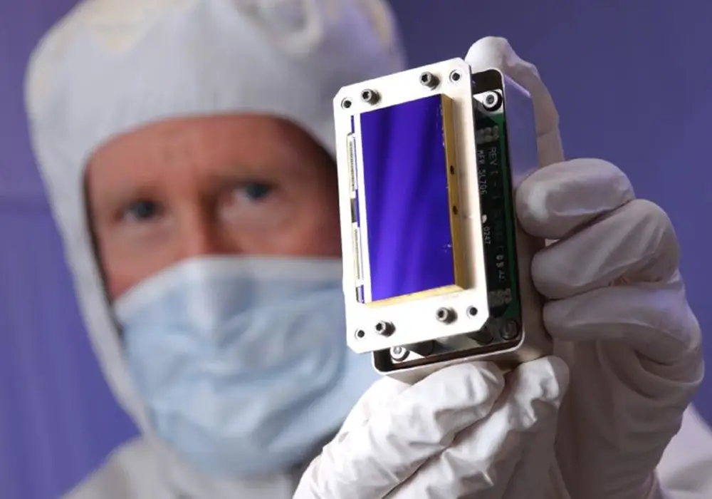
Kepler focal plane detector - CCD
One of the 42 charged couple devices (CCDs) used in the Kepler focal plane array mounted in its shipping
container. The CCDs were manufactured by Teledyne e2v Space Imaging in Chelmsford, England.
Credit: NASA and Ball Aerospace
The original Kepler mission stared continuously for 3.5 years at over 100,000 stars in the constellation Cygnus. The
Kepler mission was extended multiple times and was able to observe over 500,000 stars during a nine-year operation
that ended in 2018. With a relatively large primary mirror of 1.4-meter diameter and sensitive CCDs, Kepler (and its
follow-on mission, dubbed K2) achieved a high signal-to-noise ratio that enabled the discovery of over half of all
confirmed exoplanets discovered through April 2024. Kepler and K2 are credited with 3,322 confirmed exoplanets and
2,959 exoplanet candidates yet to be confirmed.
NASA's Kepler mission was a statistical transit survey designed to determine the frequency of Earth-sized planets
around other stars. Kepler concentrated on a relatively small region of the sky - 115 square degrees, only about
0.25% of the full sky - searching for exoplanets orbiting stars up to a distance of 3,000 light years. While Kepler
was revolutionary in its finding that Earth-to-Neptune-sized planets are common, the bulk of the stars in the Kepler
field lie at distances of hundreds to thousands of light-years, making it difficult to obtain ground-based follow-up
observations for many systems.
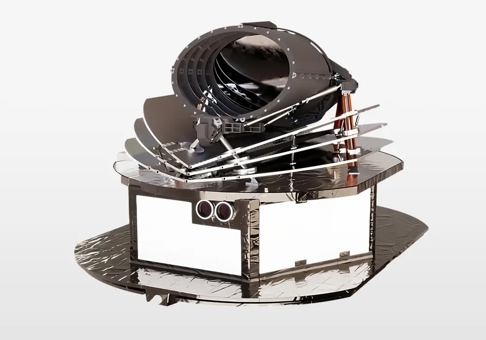
TESS: NASA's second planet-finding mission based on the transit photometry approach, named TESS, has a
different goal: observe most of the sky but only find exoplanets relatively close to the Earth. The Transiting
Exoplanet Survey Satellite (TESS) mission was designed to discover exoplanets in orbit around the brightest dwarf
stars in the sky, searching within 200 light-years of the Earth. This design trade was implemented by four
wide-field of view cameras, each with a relatively small 10.5 cm (0.105-m) aperture. The combined field of view of
the four cameras is 24x96 degrees. The TESS mission imaged about 75% of the sky during its two-year primary mission.
Launched in 2018, the TESS mission has been extended twice and is still operational. As of November 2023, TESS has
discovered at least 450 confirmed exoplanets with more than 4,500 candidate exoplanets awaiting confirmation (or
rejection) as exoplanets. (The TESS mission is operated by the Massachusetts Institute of Technology. The four
TESS cameras use a total of 16 2Kx2K frame transfer CCDs - 2Kx4K pixels each - produced by MIT Lincoln
Laboratory.)
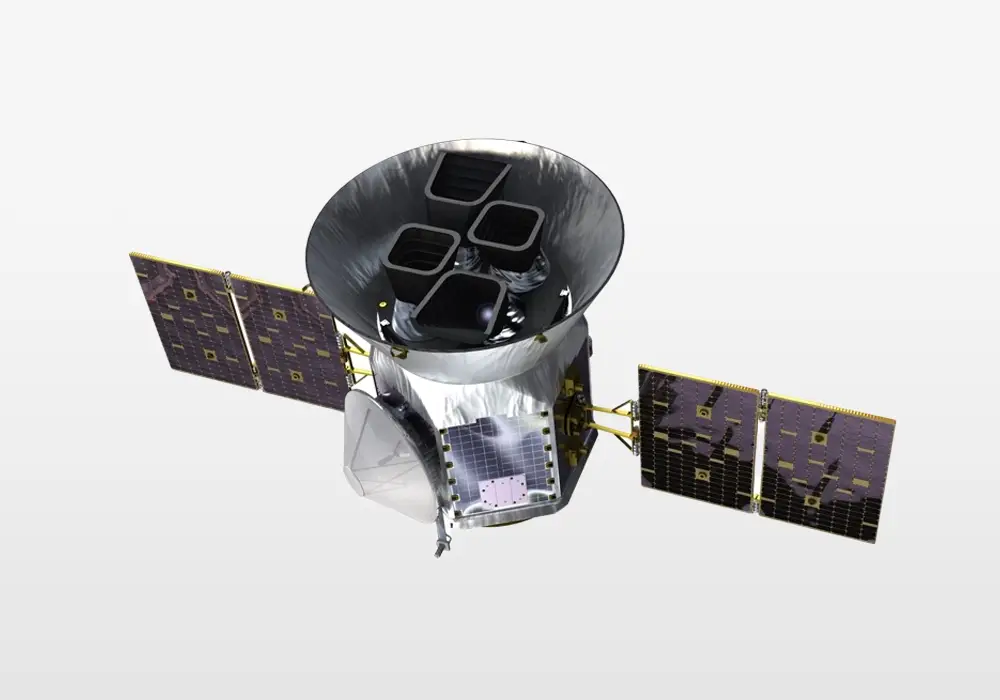
Artist's conception of the TESS spacecraft and payload
The apertures of the four cameras can be seen in the center of the image.
Credit: Massachusetts Institute of Technology (MIT)
PLATO: Not to be left behind in the hunt for exoplanets, the European Space Agency (ESA) will launch an
ambitious transit photometry mission in 2026. The PLAnetary Transits and Oscillations (PLATO) mission will
have 26 cameras to find and study terrestrial exoplanets in orbits in the habitable zones of Sun-like stars. PLATO
will be launched to Lagrange Point L2 and will observe more than 200,000 stars during its nominal four-year mission.
Each of the 26 PLATO cameras uses four Teledyne e2v CCDs; each CCD has 4510x4510 pixels (18 µm pitch). Each
camera has more than 81 million pixels, and there are a total of more than 2 billion CCD pixels in the 26 cameras of
the PLATO mission, with images taken every 25 seconds. ESA officially designated the PLATO CCDs as "CCD
Bruyères" in honor of the late Teledyne e2v employee Jean-Francois Bruyères. Jean-Francois was a
long-serving and highly respected colleague in the field of space imaging who was instrumental in the development of
CCDs for many ESA missions.
Artist's impression of the PLATO spacecraft
The apertures for the 26 cameras can be seen on the spacecraft.
Credit: ESA/ATG medialab
PLATO CCD Cameras under test and single CCD
Left: The 26 PLATO cameras integrated and under test in the cleanroom of OHB Systems AG (Bremen, Germany).
Right: One of the 104 Bruyères CCDs (4510x4510 pixels) under test at Teledyne e2v (Chelmsford, UK).
Credit: OHB, Teledyne e2v
The Holy Grail for Exoplanet Discovery and Measurement - Direct Imaging
The discovery of exoplanets using radial velocity spectroscopy was a very significant event in astronomy. Although
today we hear news stories about exoplanets on a weekly basis, before the 1990's, the existence of exoplanets was in
the realm of theory and speculation. Radial velocity spectroscopy showed us that planets can be readily found
orbiting main sequence stars. The large number of exoplanets found via transit photometry, which relies on unique
alignment of the exoplanet orbit with direction to the Earth, demonstrated that exoplanets are common. Through April
2024, over 5,600 exoplanets have been confirmed with nearly 10,000 additional exoplanet candidates identified (and
awaiting confirmation or rejection). Based on studies to date, astronomers now think there are on average one to two
exoplanets per star, with some stars having several exoplanets. That amounts to about 1 billion exoplanets in our
Milky Way galaxy. The consensus is that 20% of Sun-like stars have an Earth-sized planet in its habitable zone.
While the radial velocity and transit photometry techniques have been very useful for birthing the new
field of exoplanet science, both techniques are indirect measurements of exoplanets, requiring only measurement of the
host star light. Missions like Ariel will use transit spectroscopy, a technique that measures the light of both
the star and the exoplanet. Ariel will study hot exoplanets (gas giant, mini-Neptunes,
super-Earths) but cannot study Earth-like exoplanets orbiting Sun-like stars. For an Earth-like planet orbiting in
the habitable zone of a Sun-like star, the host star's light is 100 million (108) to 10 billion (1010)
times brighter than the exoplanet's light. The techniques of radial velocity and transit photometry will not work
for Earth analogues since the faint light from an Earth-like exoplanet will be swamped by the "photon noise" of the
much brighter Sun-like star.
- All light has statistical fluctuations. Even a "constant intensity" light source has fluctuations in the
number of photons received at Earth during a given time period. "Photon shot noise" is equal to the square
root of the number of photons.
- Since a Sun-like star is 108 to 1010 times brighter than an Earth-like exoplanet, the
photon noise of the Sun-like star is 10,000 (104) to 100,000 (105) times the signal of
the exoplanet.
- Transit spectroscopy will never be able to disentangle the light from an Earth analogue exoplanet from
the light of its host star.
The only way to study an Earth-like exoplanet for the biosignatures of life is to fully separate the exoplanet's
light, measuring it independently from its host star. The only approach that can do this is direct imaging of
the exoplanet while suppressing the light of the star with a "coronagraph". Named after optics used to study the
Sun's corona, a coronagraph is a set of optics that blocks out the direct light from a star or other bright
object, enabling the light from a faint nearby object (the exoplanet) to be measured. When used to study exoplanets,
this set of optics is sometimes called a stellar coronagraph. The concept of a stellar coronagraph is
presented in the NASA animation (see below) that explains the coronagraph in the Roman Space Telescope (RST).
Animation of the Roman Space Telescope Coronagraph Instrument
Please turn on your computer sound, unmute and hear the audio description of the animation
Credit: NASA
The RST coronagraph will reduce an exoplanet's host star light by a factor of 200 million (2x10⁸). The
coronagraph achieves this contrast ratio by using a specialized coronagraphic mask and "adaptive optics" to remove
any wavefront distortions. The Roman Space Telescope is scheduled to launch by May 2027.
For the past 20 years, coronagraphic direct imaging has been pursued by several ground-based observatories that
developed coronagraphs outfitted with adaptive optics to correct for the blurring of the Earth's atmosphere.
The first discovery of an exoplanet by direct imaging was announced in 2008 by Christian Marois of the Herzberg
Institute of Astrophysics (Canada). The Marois group used a coronagraphic instrument at the Keck Observatory
(Hawai'i) to discover three exoplanets orbiting a young star named HR 8799. The movie below, generated from data
taken over a period of 7 years at the Keck Observatory, shows four planets more massive than Jupiter orbiting HR
8799. The movie doesn't show full orbits since only partial orbits were completed over 7 years. The closest-in
exoplanet orbits the star in about 40 years; the farthest-out exoplanet takes more than 400 years. The black circle
in the center of the image is from the coronagraph blocking the blinding light of the star, making the exoplanets
visible. Star light leaking past the coronagraph mask appears as the speckle pattern outside the central black area.
The images were initially captured by Dr. Christian Marois of the National Research Council of Canada's Herzberg
Institute of Astrophysics. The movie animation was constructed by Jason Wang of the University of California,
Berkeley. The movie is based on eight observations of the exoplanets since 2009; a motion interpolation algorithm
was used to draw the orbit between those points.
Animation of a sequence of direct images taken by the Keck Observatory of the HR 8799 system
Light from the central star has been blocked by a coronagraph to enable imaging of four exoplanets. The
scale bar on the image marked "20 au" denotes 20 astronomical units (au), where 1 au is the distance of the
Earth from the Sun (93 million miles).
Credit: Jason Wang (University of California, Berkeley) and Christian Marois (National Research Council
of Canada, Herzberg Institute of Astrophysics)
HR 8799 is about 130 light-years away in the constellation of Pegasus. By coincidence, it is quite close to the star
51 Pegasi, where the first exoplanet was detected in 1995. HR 8799 is about 30 million years old and is almost five
times brighter than the Sun.
The exoplanets of HR 8799 were the first exoplanets to be directly imaged. During the past 15 years, 40 additional
exoplanets have been directly imaged by ground-based telescopes. However, it has only been possible to image large
gas exoplanets orbiting far from their host stars. The existing coronagraphs are not good enough to image Earth-like
exoplanets around Sun-like stars.
But these observations demonstrate that direct imaging of exoplanets is feasible and, in 2027, the Roman Space
Telescope coronagraph will take the next big step in this technology. The world's astronomical community is
anxiously awaiting more advanced space-based coronagraph imagers, operating above the Earth's blurring atmosphere,
to be able to directly image and spectroscopically study the atmospheres of small exoplanets orbiting close to their
host star. The July 2024 article will present the Habitable Worlds Observatory (HWO), NASA's future flagship
astrophysics mission that will launch in the late 2030's. HWO aims to achieve 1010 suppression of the
star's light to enable imaging and spectroscopy of Earth-like exoplanets. HWO will attempt to answer the age old
question "Are we alone?".
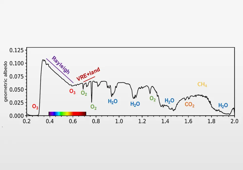
Reflected sunlight spectrum of the Earth's atmosphere
Biosignature of the "Modern Earth" atmosphere which has been in existence for 540 million years
Credit: NASA
The Earth has been in existence for about 4.6 billion years with the Earth's history roughly divided into four different
eras during which the Earth's atmosphere evolved:
- 600 million years in the "Hadean" era
- 1,500 million years in the "Archean" era
- 2,000 million years in the "Proterozoic" era
- 540 million years in the "Modern" era
Postscript
This article discussed only a few of the methods by which exoplanets are discovered, with focus on:
- Radial Velocity
- Transit Photometry
- Direct Imaging
Several other methods to find exoplanets were not presented. But one method that deserves mentioning is gravitational microlensing. Gravitational microlensing occurs when the gravitational field of a star acts like a lens, magnifying the light of a more distant background star. This effect can occur when the two stars are almost exactly aligned. Lensing events are brief, lasting for weeks or days, as the two stars and Earth are all moving relative to each other. Over the past ten years, 217 exoplanets have been discovered by gravitational microlensing.
If the foreground lensing star has an exoplanet, then the exoplanet's own gravitational field can make a detectable contribution to the lensing effect. Since gravitational microlensing from an exoplanet requires a highly unlikely alignment, a very large number of distant stars must be continuously monitored in order to detect an exoplanetary microlensing event. Gravitational microlensing is most fruitful for exoplanets that are located between the Earth and the center of the Milky Way galaxy, as the galactic center provides a large number of background stars.
The Roman Space Telescope has an observational program labeled the "Galactic Bulge Time-Domain Survey" that will scour the center of the Milky Way for microlensing events. This survey will provide one of the deepest views ever into the heart of our galaxy, making observations every 15 minutes for over a year. Tracking how hundreds of millions of stars change in brightness is predicted to discover up to 100,000 exoplanets and find isolated black holes.

